This chapter describes partitioned tables and indexes. It covers the following topics:
Partitioning addresses key
issues in supporting very large tables and indexes by letting you
decompose them into smaller and more manageable pieces called partitions.
SQL queries and DML statements do not need to be modified in order to
access partitioned tables. However, after partitions are defined, DDL
statements can access and manipulate individuals partitions rather than
entire tables or indexes. This is how partitioning can simplify the
manageability of large database objects. Also, partitioning is entirely
transparent to applications.
Each partition of a table or index must have the same
logical attributes, such as column names, datatypes, and constraints,
but each partition can have separate physical attributes such as
pctfree, pctused, and tablespaces.
Partitioning is useful for many different types of
applications, particularly applications that manage large volumes of
data. OLTP systems often benefit from improvements in manageability and
availability, while data warehousing systems benefit from performance
and manageability.
Note:
All partitions of a partitioned object must reside in tablespaces of a single block size.
|
Partitioning offers these advantages:
Figure 11-1 offers a graphical view of how partitioned tables differ from nonpartitioned tables.
Figure 11-1 A View of Partitioned Tables
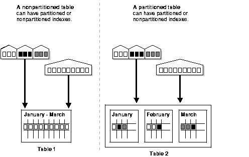
Text description of the illustration cncpt162.gif
Partition Key
Each row in a partitioned table is unambiguously assigned
to a single partition. The partition key is a set of one or more columns
that determines the partition for each row. Oracle9i
automatically directs insert, update, and delete operations to the
appropriate partition through the use of the partition key. A partition
key:
- Consists of an ordered list of 1 to 16 columns
- Cannot contain a
LEVEL, ROWID, or MLSLABEL pseudocolumn or a column of type ROWID - Can contain columns that are
NULLable
Partitioned Tables
Tables can be partitioned into up to 64,000 separate
partitions. Any table can be partitioned except those tables containing
columns with LONG or LONG RAW datatypes. You can, however, use tables containing columns with CLOB or BLOB datatypes.
Partitioned Index-Organized Tables
You can range partition index-organized tables. This
feature is very useful for providing improved manageability,
availability and performance for index-organized tables. In addition,
data cartridges that use index-organized tables can take advantage of
the ability to partition their stored data. Common examples of this are
the Image and interMedia cartridges.
For partitioning an index-organized table:
- Only range and hash partitioning are supported
- Partition columns must be a subset of primary key columns
- Secondary indexes can be partitioned -- locally and globally
OVERFLOW data segments are always equipartitioned with the table partitions
Oracle provides the following partitioning methods:
Figure 11-2 offers a graphical view of the methods of partitioning.
Figure 11-2 List, Range, and Hash Partitioning
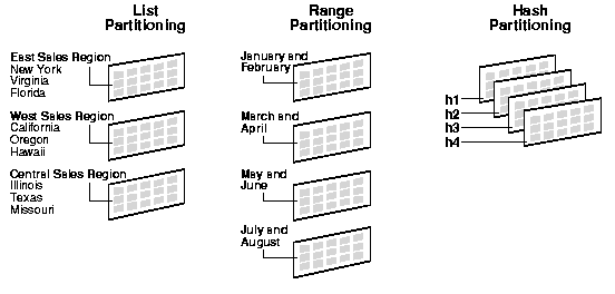
Text description of the illustration cncpt158.gif
Composite partitioning is a combination of other
partitioning methods. Oracle currently supports range-hash and
range-list composite partitioning. Figure 11-3 offers a graphical view of range-hash and range-list composite partitioning.
Figure 11-3 Composite Partitioning
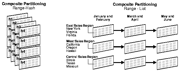
Text description of the illustration cncpt168.gif
Range Partitioning
Range partitioning maps data to partitions based on ranges
of partition key values that you establish for each partition. It is
the most common type of partitioning and is often used with dates. For
example, you might want to partition sales data into monthly partitions.
When using range partitioning, consider the following rules:
- Each partition has a
VALUES LESS THAN
clause, which specifies a noninclusive upper bound for the partitions.
Any binary values of the partition key equal to or higher than this
literal are added to the next higher partition. - All partitions, except the first, have an implicit lower bound specified by the
VALUES LESS THAN clause on the previous partition. - A
MAXVALUE literal can be defined for the highest partition. MAXVALUE
represents a virtual infinite value that sorts higher than any other
possible value for the partition key, including the null value.
A typical example is given in the following section. The statement creates a table (sales_range) that is range partitioned on the sales_date field.
Range Partitioning Example
CREATE TABLE sales_range
(salesman_id  NUMBER(5),
salesman_name VARCHAR2(30),
sales_amount  NUMBER(10),
sales_date    DATE)
PARTITION BY RANGE(sales_date)
(
PARTITION sales_jan2000 VALUES LESS THAN(TO_DATE('02/01/2000','DD/MM/YYYY')),
PARTITION sales_feb2000 VALUES LESS THAN(TO_DATE('03/01/2000','DD/MM/YYYY')),
PARTITION sales_mar2000 VALUES LESS THAN(TO_DATE('04/01/2000','DD/MM/YYYY')),
PARTITION sales_apr2000 VALUES LESS THAN(TO_DATE('05/01/2000','DD/MM/YYYY'))
);
List Partitioning
List partitioning enables you to explicitly control how
rows map to partitions. You do this by specifying a list of discrete
values for the partitioning key in the description for each partition.
This is different from range partitioning, where a range of values is
associated with a partition and from hash partitioning, where a hash
function controls the row-to-partition mapping. The advantage of list
partitioning is that you can group and organize unordered and unrelated
sets of data in a natural way.
The details of list partitioning can best be described
with an example. In this case, let's say you want to partition a sales
table by region. That means grouping states together according to their
geographical location as in the following example.
List Partitioning Example
CREATE TABLE sales_list
(salesman_id  NUMBER(5),
salesman_name VARCHAR2(30),
sales_state   VARCHAR2(20),
sales_amount  NUMBER(10),
sales_date    DATE)
PARTITION BY LIST(sales_state)
(
PARTITION sales_west VALUES('California', 'Hawaii'),
PARTITION sales_east VALUES ('New York', 'Virginia', 'Florida'),
PARTITION sales_central VALUES('Texas', 'Illinois')
PARTITION sales_other VALUES(DEFAULT)
);
A row is mapped to a partition by checking whether the
value of the partitioning column for a row falls within the set of
values that describes the partition. For example, the rows are inserted
as follows:
- (
10, 'Jones', 'Hawaii', 100, '05-JAN-2000') maps to partition sales_west - (
21, 'Smith', 'Florida', 150, '15-JAN-2000') maps to partition sales_east - (
32, 'Lee', 'Colorado', 130, '21-JAN-2000') does not map to any partition in the table
Unlike range and hash partitioning, multicolumn partition
keys are not supported for list partitioning. If a table is partitioned
by list, the partitioning key can only consist of a single column of the
table.
The DEFAULT partition enables you to avoid
specifying all possible values for a list-partitioned table by using a
default partition, so that all rows that do not map to any other
partition do not generate an error.
Hash Partitioning
Hash partitioning enables easy partitioning of data that
does not lend itself to range or list partitioning. It does this with a
simple syntax and is easy to implement. It is a better choice than range
partitioning when:
- You do not know beforehand how much data maps into a given range
- The sizes of range partitions would differ quite substantially or would be difficult to balance manually
- Range partitioning would cause the data to be undesirably clustered
- Performance features such as parallel DML, partition pruning, and partition-wise joins are important
The concepts of splitting, dropping or merging partitions
do not apply to hash partitions. Instead, hash partitions can be added
and coalesced.
Hash Partitioning Example
CREATE TABLE sales_hash
(salesman_id  NUMBER(5),
salesman_name VARCHAR2(30),
sales_amount  NUMBER(10),
week_no       NUMBER(2))
PARTITION BY HASH(salesman_id)
PARTITIONS 4
STORE IN (data1, data2, data3, data4);
The preceding statement creates a table sales_hash, which is hash partitioned on salesman_id field. The tablespace names are data1, data2, data3, and data4.
Composite Partitioning
Composite partitioning partitions data using the range
method, and within each partition, subpartitions it using the hash or
list method. Composite range-hash partitioning provides the improved
manageability of range partitioning and the data placement, striping,
and parallelism advantages of hash partitioning. Composite range-list
partitioning provides the manageability of range partitioning and the
explicit control of list partitioning for the subpartitions.
Composite partitioning supports historical operations,
such as adding new range partitions, but also provides higher degrees of
parallelism for DML operations and finer granularity of data placement
through subpartitioning.
Composite Partitioning Range-Hash Example
CREATE TABLE sales_composite
(salesman_id  NUMBER(5),
 salesman_name VARCHAR2(30),
 sales_amount  NUMBER(10),
 sales_date    DATE)
PARTITION BY RANGE(sales_date)
SUBPARTITION BY HASH(salesman_id)
SUBPARTITION TEMPLATE(
SUBPARTITION sp1 TABLESPACE data1,
SUBPARTITION sp2 TABLESPACE data2,
SUBPARTITION sp3 TABLESPACE data3,
SUBPARTITION sp4 TABLESPACE data4)
(PARTITION sales_jan2000 VALUES LESS THAN(TO_DATE('02/01/2000','DD/MM/YYYY'))
 PARTITION sales_feb2000 VALUES LESS THAN(TO_DATE('03/01/2000','DD/MM/YYYY'))
 PARTITION sales_mar2000 VALUES LESS THAN(TO_DATE('04/01/2000','DD/MM/YYYY'))
 PARTITION sales_apr2000 VALUES LESS THAN(TO_DATE('05/01/2000','DD/MM/YYYY'))
 PARTITION sales_may2000 VALUES LESS THAN(TO_DATE('06/01/2000','DD/MM/YYYY')));
This statement creates a table sales_composite that is range partitioned on the sales_date field and hash subpartitioned on salesman_id.
When you use a template, Oracle names the subpartitions by
concatenating the partition name, an underscore, and the subpartition
name from the template. Oracle places this subpartition in the
tablespace specified in the template. In the previous statement, sales_jan2000_sp1 is created and placed in tablespace data1 while sales_jan2000_sp4 is created and placed in tablespace data4. In the same manner, sales_apr2000_sp1 is created and placed in tablespace data1 while sales_apr2000_sp4 is created and placed in tablespace data4. Figure 11-4 offers a graphical view of the previous example.
Figure 11-4 Composite Range-Hash Partitioning
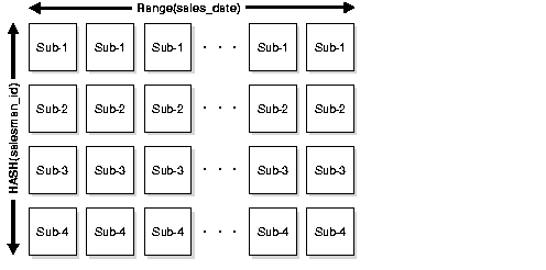
Text description of the illustration cncpt157.gif
Composite Partitioning Range-List Example
CREATE TABLE bimonthly_regional_sales
(deptno NUMBER,
 item_no VARCHAR2(20),
 txn_date DATE,
 txn_amount NUMBER,
 state VARCHAR2(2))
PARTITION BY RANGE (txn_date)
SUBPARTITION BY LIST (state)
SUBPARTITION TEMPLATE(


SUBPARTITION east VALUES('NY', 'VA', 'FL') TABLESPACE ts1,
SUBPARTITION west VALUES('CA', 'OR', 'HI') TABLESPACE ts2,
SUBPARTITION central VALUES('IL', 'TX', 'MO') TABLESPACE ts3)
(
PARTITION janfeb_2000 VALUES LESS THAN (TO_DATE('1-MAR-2000','DD-MON-YYYY')),
PARTITION marapr_2000 VALUES LESS THAN (TO_DATE('1-MAY-2000','DD-MON-YYYY')),
PARTITION mayjun_2000 VALUES LESS THAN (TO_DATE('1-JUL-2000','DD-MON-YYYY'))
);
This statement creates a table bimonthly_regional_sales that is range partitioned on the txn_date field and list subpartitioned on state.
When you use a template, Oracle names the subpartitions by
concatenating the partition name, an underscore, and the subpartition
name from the template. Oracle places this subpartition in the
tablespace specified in the template. In the previous statement, janfeb_2000_east is created and placed in tablespace ts1 while janfeb_2000_central is created and placed in tablespace ts3. In the same manner, mayjun_2000_east is placed in tablespace ts1 while mayjun_2000_central is placed in tablespace ts3. Figure 11-5 offers a graphical view of the table bimonthly_regional_sales and its 9 individual subpartitions.
Figure 11-5 Composite Range-List Partitioning
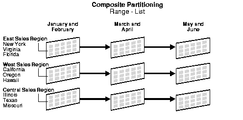
Text description of the illustration cncpt167.gif
When to Partition a Table
Here are some suggestions for when to partition a table:
- Tables greater than 2GB should always be considered for partitioning.
- Tables containing
historical data, in which new data is added into the newest partition. A
typical example is a historical table where only the current month's
data is updatable and the other 11 months are read-only.
Just like partitioned tables, partitioned indexes improve
manageability, availability, performance, and scalability. They can
either be partitioned independently (global indexes) or automatically
linked to a table's partitioning method (local indexes).
Local Partitioned Indexes
Local partitioned indexes are easier to manage than other
types of partitioned indexes. They also offer greater availability and
are common in DSS environments. The reason for this is equipartitioning:
each partition of a local index is associated with exactly one
partition of the table. This enables Oracle to automatically keep the
index partitions in sync with the table partitions, and makes each
table-index pair independent. Any actions that make one partition's data
invalid or unavailable only affect a single partition.
You cannot explicitly add a partition to a local index.
Instead, new partitions are added to local indexes only when you add a
partition to the underlying table. Likewise, you cannot explicitly drop a
partition from a local index. Instead, local index partitions are
dropped only when you drop a partition from the underlying table.
A local index can be unique. However, in order for a local
index to be unique, the partitioning key of the table must be part of
the index's key columns. Unique local indexes are useful for OLTP
environments.
Figure 11-6 offers a graphical view of local partitioned indexes.
Figure 11-6 Local Partitioned Index
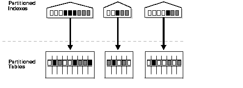
Text description of the illustration cncpt161.gif
Global Partitioned Indexes
Global partitioned indexes are flexible in that the degree
of partitioning and the partitioning key are independent from the
table's partitioning method. They are commonly used for OLTP
environments and offer efficient access to any individual record.
The highest partition of a global index must have a partition bound, all of whose values are MAXVALUE.
This ensures that all rows in the underlying table can be represented
in the index. Global prefixed indexes can be unique or nonunique.
You cannot add a partition to a global index because the highest partition always has a partition bound of MAXVALUE. If you wish to add a new highest partition, use the ALTER INDEX SPLIT PARTITION statement. If a global index partition is empty, you can explicitly drop it by issuing the ALTER INDEX DROP PARTITION
statement. If a global index partition contains data, dropping the
partition causes the next highest partition to be marked unusable. You
cannot drop the highest partition in a global index.
Maintenance of Global Partitioned Indexes
By default, the following operations on partitions on a heap-organized table mark all global indexes as unusable:
ADD (HASH)
COALESCE (HASH)
DROP
EXCHANGE
MERGE
MOVE
SPLIT
TRUNCATE
These indexes can be maintained by appending the clause UPDATE GLOBAL INDEXES to the SQL statements for the operation. The two advantages to maintaining global indexes:
- The index remains available and online throughout the operation. Hence no other applications are affected by this operation.
- The index doesn't have to be rebuilt after the operation.
Example:
ALTER TABLE DROP PARTITION P1 UPDATE GLOBAL INDEXES
Note:
This feature is supported only for heap organized tables.
|
Figure 11-7 offers a graphical view of global partitioned indexes.
Figure 11-7 Global Partitioned Index
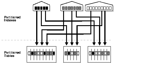
Text description of the illustration cncpt160.gif
Global Nonpartitioned Indexes
Global nonpartitioned indexes behave just like a
nonpartitioned index. They are commonly used in OLTP environments and
offer efficient access to any individual record.
Figure 11-8 offers a graphical view of global nonpartitioned indexes.
Figure 11-8 Global Nonpartitioned Index
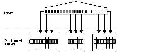
Text description of the illustration cncpt159.gif
Partitioned Index Examples
Example of Index Creation: Starting Table Used for Examples
CREATE TABLE employees
(employee_id NUMBER(4) NOT NULL,
 last_name VARCHAR2(10),
 department_id NUMBER(2))
PARTITION BY RANGE (department_id)
(PARTITION employees_part1 VALUES LESS THAN (11) TABLESPACE part1,
 PARTITION employees_part2 VALUES LESS THAN (21) TABLESPACE part2,
 PARTITION employees_part3 VALUES LESS THAN (31) TABLESPACE part3);
Example of a Local Index Creation
CREATE INDEX employees_local_idx ON employees (employee_id) LOCAL;
Example of a Global Index Creation
CREATE INDEX employees_global_idx ON employees(employee_id);
Example of a Global Partitioned Index Creation
CREATE INDEX employees_global_part_idx ON employees(employee_id)
GLOBAL PARTITION BY RANGE(employee_id)
(PARTITION p1 VALUES LESS THAN(5000),
 PARTITION p2 VALUES LESS THAN(MAXVALUE));
Example of a Partitioned Index-Organized Table Creation
CREATE TABLE sales_range
(
salesman_id   NUMBER(5),
salesman_name VARCHAR2(30),
sales_amount  NUMBER(10),
sales_date    DATE,
PRIMARY KEY(sales_date, salesman_id))
ORGANIZATION INDEX INCLUDING salesman_id
OVERFLOW TABLESPACE tabsp_overflow
PARTITION BY RANGE(sales_date)
(PARTITION sales_jan2000 VALUES LESS THAN(TO_DATE('02/01/2000','DD/MM/YYYY'))
 OVERFLOW TABLESPACE p1_overflow,
 PARTITION sales_feb2000 VALUES LESS THAN(TO_DATE('03/01/2000','DD/MM/YYYY'))
 OVERFLOW TABLESPACE p2_overflow,
 PARTITION sales_mar2000 VALUES LESS THAN(TO_DATE('04/01/2000','DD/MM/YYYY'))
 OVERFLOW TABLESPACE p3_overflow,
 PARTITION sales_apr2000 VALUES LESS THAN(TO_DATE('05/01/2000','DD/MM/YYYY'))
 OVERFLOW TABLESPACE p4_overflow);
Miscellaneous Information about Creating Indexes on Partitioned Tables
You can create bitmap indexes on partitioned tables, with
the restriction that the bitmap indexes must be local to the partitioned
table. They cannot be global indexes.
Global indexes can be unique. Local indexes can only be unique if the partitioning key is a part of the index key.
Using Partitioned Indexes in OLTP Applications
Here are a few guidelines for OLTP applications:
- Global indexes and
unique, local indexes provide better performance than nonunique local
indexes because they minimize the number of index partition probes.
- Local indexes offer better availability when there are partition or subpartition maintenance operations on the table.
Using Partitioned Indexes in Data Warehousing and DSS Applications
Here are a few guidelines for data warehousing and DSS applications:
- Local indexes are preferable because they are easier to manage during data loads and during partition-maintenance operations.
- Local indexes can
improve performance because many index partitions can be scanned in
parallel by range queries on the index key.
Partitioned Indexes on Composite Partitions
Here are a few points to remember when using partitioned indexes on composite partitions:
- Only range partitioned global indexes are supported.
- Subpartitioned indexes are always local and stored with the table subpartition by default.
- Tablespaces can be specified at either index or index subpartition levels.
Partitioning can help you improve performance and
manageability. Some topics to keep in mind when using partitioning for
these reasons are:
Partition Pruning
The Oracle server explicitly recognizes partitions and
subpartitions. It then optimizes SQL statements to mark the partitions
or subpartitions that need to be accessed and eliminates (prunes)
unnecessary partitions or subpartitions from access by those SQL
statements. In other words, partition pruning is the skipping of
unnecessary index and data partitions or subpartitions in a query.
For each SQL statement, depending on the selection
criteria specified, unneeded partitions or subpartitions can be
eliminated. For example, if a query only involves March sales data, then
there is no need to retrieve data for the remaining eleven months. Such
intelligent pruning can dramatically reduce the data volume, resulting
in substantial improvements in query performance.
If the optimizer determines that the selection criteria
used for pruning are satisfied by all the rows in the accessed partition
or subpartition, it removes those criteria from the predicate list (WHERE
clause) during evaluation in order to improve performance. However, the
optimizer cannot prune partitions if the SQL statement applies a
function to the partitioning column (with the exception of the TO_DATE
function). Similarly, the optimizer cannot use an index if the SQL
statement applies a function to the indexed column, unless it is a
function-based index.
Pruning can eliminate index partitions even when the
underlying table's partitions cannot be eliminated, but only when the
index and table are partitioned on different columns. You can often
improve the performance of operations on large tables by creating
partitioned indexes that reduce the amount of data that your SQL
statements need to access or modify.
Equality, range, LIKE, and IN-list predicates are considered for partition pruning with range or list partitioning, and equality and IN-list predicates are considered for partition pruning with hash partitioning.
Partition Pruning Example
We have a partitioned table called orders. The partition key for orders is order_date. Let's assume that orders has six months of data, January to June, with a partition for each month of data. If the following query is run:
SELECT SUM(value)
FROM orders
WHERE order_date BETWEEN '28-MAR-98' AND '23-APR-98'
Partition pruning is achieved by:
- First, partition elimination of January, February, May, and June data partitions. Then either:
- An index scan of the March and April data partition due to high index selectivity
or
- A full scan of the March and April data partition due to low index selectivity
Partition-wise Joins
A partition-wise join is a join optimization that you can
use when joining two tables that are both partitioned along the join
column(s). With partition-wise joins, the join operation is broken into
smaller joins that are performed sequentially or in parallel. Another
way of looking at partition-wise joins is that they minimize the amount
of data exchanged among parallel slaves during the execution of parallel
joins by taking into account data distribution.
Parallel DML
Parallel execution dramatically reduces response time for
data-intensive operations on large databases typically associated with
decision support systems and data warehouses. In addition to
conventional tables, you can use parallel query and parallel DML with
range- and hash-partitioned tables. By doing so, you can enhance
scalability and performance for batch operations.
The semantics and restrictions for parallel DML sessions are the same whether you are using index-organized tables or not.
See Also:
Oracle9i Data Warehousing Guide for more information about parallel DML and its use with partitioned tables